I was recently showed the fantasic site wxchats.eu by a friend. This site displays data from various NWP models and forecasts. Playing with during the recent cold snap got me wondering where they got their data from. I found one agency, The German Weather Service, which provides large amounts of its data freely on their opendata site. Their ICON-EU forecast covers all of Europe (and some more besides) so I decided to try and look at how I could visualise this and potentially process it using some code.
Grib2 and Panoply
The data is distributed in a binary format called GRIB2. This format is used for efficient representation of gridded data. We can download a grib2 file from the opendata site and view it by navigating through the directories to /weather/icon/eu_nest/grib/. This shows a list of two digit numbers which represent when the model was run, for example 06 means that the model was run at 6am. Inside a specific run you will see all the different types of things they forecast: precipitation, temperature, etc… You can see all of the different types of forecasts they have in this pdf.
For this project I want to try and read the forecasted 2m temperature, so I will navigate to the t_2m folder. There you will see all of the different grib2 files. Each file represents the forecasted data for a different hour after the forecast was run. The file names use the following pattern: ICON_EU_single_level_elements_T_2M_YYYYMMDDRR_HHH.grib2.bz2. Here RR is the two digit run code (eg 06 or 12) and HHH is the number of hours since the model was run the file is forecasting.
If you download one of those and extract the grib2 file. You can now open this file with a suitable application. I like to use Panoply from Nasa. With this application you can load the file, have a look at the structur of a grib file and plot some of the data. Plotting the Temperature_height_above_ground variable gives this nice map:
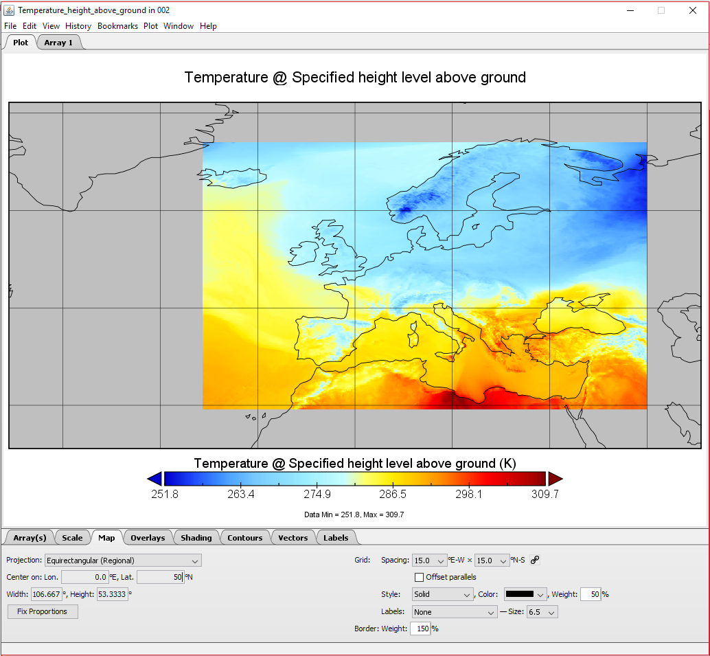
An example definition of the 2D temperature array can be seen bellow:
float Temperature_height_above_ground(time=1, height_above_ground=1, lat=657, lon=1097);
  :long_name = "Temperature @ Specified height level above ground";
  :units = "K";
  :description = "Temperature";
  :missing_value = NaNf; // float
  :grid_mapping = "LatLon_Projection";
  :coordinates = "reftime time height_above_ground lat lon ";
  :Grib_Variable_Id = "VAR_0-0-0_L103";
  :Grib2_Parameter = 0, 0, 0; // int
  :Grib2_Parameter_Discipline = "Meteorological products";
  :Grib2_Parameter_Category = "Temperature";
  :Grib2_Parameter_Name = "Temperature";
  :Grib2_Level_Type = 103; // int
  :Grib2_Level_Desc = "Specified height level above ground";
  :Grib2_Generating_Process_Type = "Forecast";
Most of the meta-data is self-describing, but the first line where you see (time=1, height_above_ground=1, lat=657, lon=1097) defines the dimensions of the data. As you can see this has four dimensions, not the expected two, but here the time and height_above_ground dimensions have size one and so we dont need to really worry about them.
Parsing the Data with Scala (or Java)
To parse the data in scala I’m going to use a java library called NetCDF. This library is designed for reading gridded data just like our GRIB2 files. In fact this library pretty much just works. With a temperature file downloaded and saved as HHH.grib2 we can use the following code to extract the forecasted temperature at a given location:
def forecast_temperature(lat: Double, long: Double, hour: String): Double = {

    val y = ((lat - 29.5) / 0.0625).toInt % 657
    val x = ((long - 336.5) / 0.0625).toInt % 1097

    val path = s"$TEMP_PATH/$hour.grib2"
    val array = NetcdfDataset.openDataset(path).findVariable("Temperature_height_above_ground").read()
    val idx = array.getIndex

    array.getDouble(idx.set(0,0,y,x)) - 273

}
Passed in a latitude and longitude this function first calulates the nearest index to search the array. The magic numbers are found as follows:
29.5- The lowest latitude that the ICON-EU model extends to (corresponds toy=0)336.5- The lowest longitude that the model extends to (corresponds tox=0)0.0625- The size of the grid squares in degrees657and1097- The respective sizes of the array. This makes sure that inputs outside of the range “wrap around” - This may or may not be a desirable feature
Once you have a dataset (NetcdfDataset.openDataset(path)) you search for a specific variable and read it to an array. This array is indexed using some strange index class (array.getIndex) which can then be used to find specific points in the array. The coordinates are 0,0,y,x where the leading zeros correspond to the time and height above ground. As you can see in the definition of the data, these are of dimension one so the only index is 0.